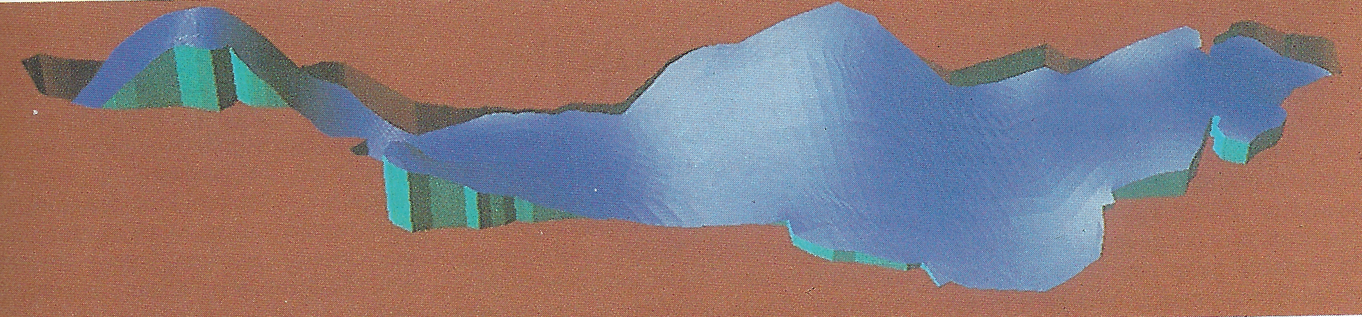
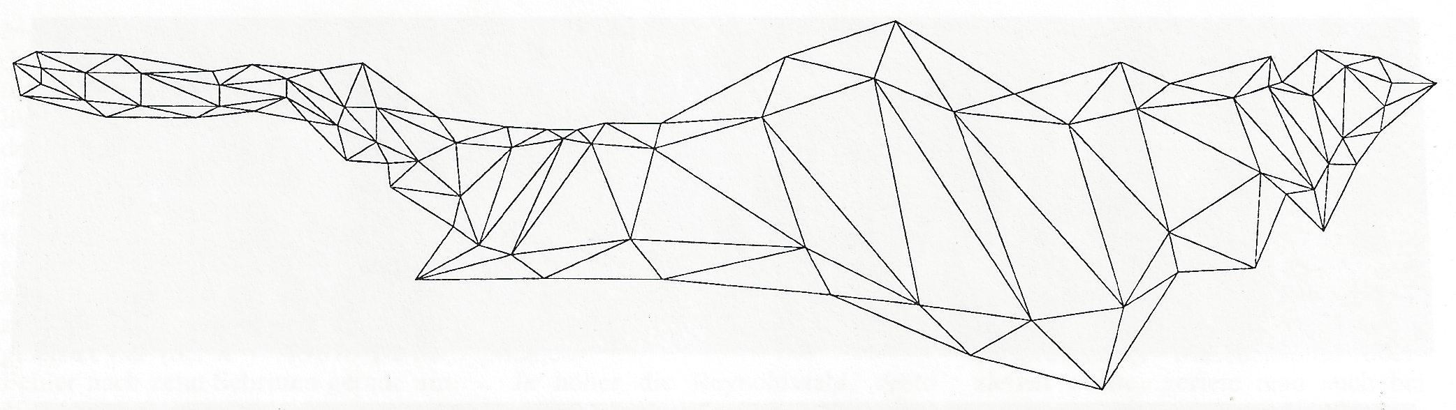
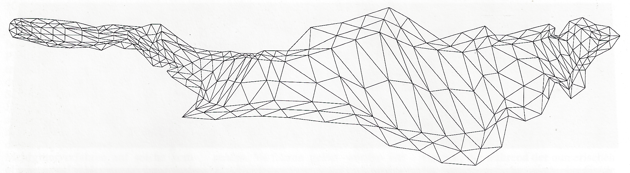
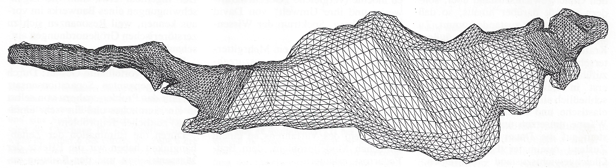
This is the (1/720) hertz eigenform of lake constance, 1 period = 12 minutes. It was computed 1990 by Sauter and Wittum, using a sequence of meshes. level 0 level 1 level 4 Multigrid Methods were very famous from 1985 until 1995. The idea was to solve the linear system which arises from Finite Element discretization as fast as possible. Let the vector space of the Finite Element functions be of dimension N. The linear system then is of (size constant * N)**2 . The matrix is sparse i.e. the number of non-zero entries of the matrix is constant * N. Multiply Matrix * Vector then takes constant * N operations. But mostly (e.g. linear static analysis) we have to solve the inverse Problem. (given A,b solve for x. Forward is A*b=x, inverse is A*x = b ). Now we see that constant * N is the lower bound of the number of operations for computing A*x = b . An explicit time step in dynamic analysis takes constant * N operatons, but the number of time steps is huge. Direct (Gaussian) Methods take constant * N**q Operations and q > 1.0 THE QUESTION IS: IS THERE ANY OPTIMAL METHOD ? THE ANSWER IS: YES but two restrictions: first: instead of constant * N we have constant * N * log N Operations. But log N increases slowly. second: We have to use special FE spaces: Nested, hierarchical, Multigrid. Since 1994 automatic meshing by Delaunay's Method became popular. But these meshes did not fit to the requirements of the FE spaces for the OPTIMAL METHOD. In 2002 the first BCC meshes came into the discussion of mesh generation methods. These FE spaces are nested, hierarchical, Multigrid. They distinguish from the traditional Multigrid meshing idea in one point: Part boundaries are fixed in the last refinement step. 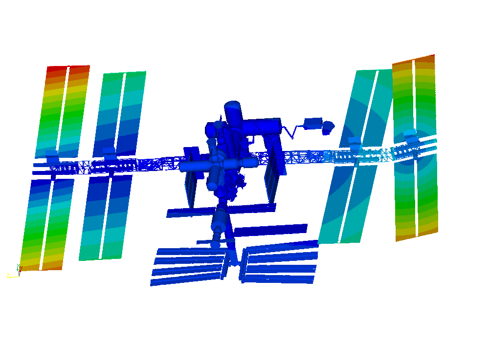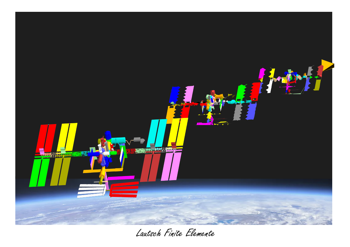4 meshes from the MMT hierarchy This is the 0.072 hertz Eigenform of our data of the International Space Station. Now I ask: is this algorithm Multigrid? HOME contact michael.lautsch[at]lautsch-fe.com